Analytics on the New York rental market | Top 15% on Kaggle!

29 Apr 2017 . category: math . Comments
#kaggle #data science #report

This is a documentation of my first serious take on a Kaggle competition - Renthop rental inquiries. Two and a half months, 146 git commits and 87 submissions later, i stand within the Top 15% on the leaderboard – A position i’m proud of!

The Kaggle competition was organized by Renthop, a rental website specific only to the New York market. Given various listing parameters like price, location, manager(broker), building, images, we had to predict the interest(internet traffic) each rental listing would receive. The “interest_listing” is a discrete variable, partitioned into “high”, “medium” and “low”.

The domain of this competition intrigued me quite a bit – Just 4 months ago, i was frustrated finding a decent place in the real estate chaos that Bangalore is! Add to that the highly competitive NY market, we have a real-world problem waiting to be solved.

My Journey - For me, this competition has been a real roller coaster – There was definitely a positive correlation between my mood and my leaderboard position! I’ve learnt a lot though, from crazy feature engineering to implementing new algorithms, from fixing validation leaks to building my custom stacker-ensemble, the learnings serve as a good jumping board for future competitions.

That being said, this blog is gonna be slightly technical. Leave if you may ;)

Till now, my standard approach towards building predictive models was to spin up a random forest on the standard variables. Not a lot of exploration or feature engineering – this approach didn’t give me dividends. In this competition, i spent the first two months understanding the features, and playing around with their combinations!

Feature Engineering

Price - One of the most obvious features is the price(logarithm of the price) of the rental listing, which leads to a better measure – Price per Room. When combined with other variables like neighborhood or street, price acts as a good proxy for “Is this the best apartment on 21st Street?”. This feature was a little tricky with studio apartments though, which have zero bedrooms by definition.

Managers - The New York market values managers(or brokers) as highly credible sources, as was visible with the nexus of brokers’ agencies. Since the manager_id was a highly categorical variable, fellow kagglers came up with an ingenious feature – “manager_score”! It is basically a combination of that manager’s percentage of “high interest” listings and “medium interest” listings. This was the most important feature in almost all of my models.

I came up with the concept of “manager_opportunity”, which indicated how good a manager’s listing was w.r.t other listings via the same manager. Basically, pitting a rental’s price against the median price of that manager – “Do you have a cheaper 2BHK apartment, Mr. Brown?”

Buildings - This feature should have been a killer one, as this is as narrow as we can get when talking about localities. I tried mapping features like “building_score”, “building_opportunity”, “building_count”, but all of them ditched my CV score. A lot of kagglers also experienced the same, and the most probable reason seems to be bad data points – 16.8% of the buildings had building_id ‘0’, though they had different coordinates. However, a positive insight out of buildings was that 90% of buildings with the “zero building_id” were of “Low Interest”, crucial!

Neighborhood - Plain old latitude and longitude turned out to be fairly important features, but we didn’t stop there :) A simple k-means with 60 clusters gave me broad neighborhoods to play with, resulting in features like “neighborhood_score” and “neighborhood_opportunity”. Initially, i’d used Google API for mapping coordinates to broad localities(as mentioned on Renthop’s website).

As i was building more and more features, i noticed a common theme – Price and Interest were the central pieces, while “Manager”, “Neighborhood”, “Building”, “Street Address”, “Time of post” were the peripheral pieces. The peripheral pieces, when integrated with a central piece via a median(or count, or generalization of some kind) gave significant improvements. This diagram was my go-to for the rest of the days :)

Street/Display Address - There were two kinds of addresses provided, street_address and display_address, which is some kind of a stripped form of street_address. I tried features like “apartment_count_on_street”(How popular is this street for rentals?) and the generic “street_opportunity”.

Another idea i pursued with street addresses was whether they contained “street number”, which should give it a boost for “exactness of address”(a variable that Renthop cares for!). Didn’t turn out to be very helpful.

A borrowed idea from a fellow kaggler – String Difference b/w the street_address and the display_addres. It was giving a sizeable difference in the “High Interest”, not a clear idea why!

Time of Post - Of course, being a seasonal business time-based features came in handy(mday, wday, hour, minutes). We couldn’t explore yearly seasonality as the dataset was sandwiched between April ‘16 and June ‘16.

It is reported that a listing on Renthop stays available for 5-6 minutes, which is highly competitive! This prompted me to look at which were the listing posted in the same hour, resulting in “hour_opportunity”(Is there a cheaper apartment posted within the last 30 minutes?”). This feature didn’t give improvement, though a similar one was useful – “hour_frequency”(number of listings posted in that hour). It probably plays to the volume of consumers online during certain times of the day.

Listing_Id - This is just a plain serial number, or so i thought! Turned out to be a very important feature, as it was surprisingly correlated with the “created” variable. Also, there were some outlier listings, which had a fairly higher listing_id than the median listing_id for rentals posted on the same date. And a high percentage of these outliers were of “Low interest”, the jury is divided on why!

Any which ways, this was an incredible insight – Sometimes, the serial id might have a lot to do with other variables!

Description - This was supposedly a treasure of minute details regarding the apartment, like “pets allowed”, “doorman”, “elevetor” amongst others. Many tried the famous tfidf algorithm, but to no avail – My hypothesis is that people initially show interest on the basis of price, location and manager. The details are considered at a later stage of renting(just before finalizing?).

A couple of features that i came up with were related to identifying spam in the descriptions – Probably, i was the first in the competition to make them public :) Calculated the percentage of capitalized letters, and number of exclamation marks – “!!DO YOU LIKE THIS DESCRIPTION?!!”

I also tried factoring in the presence of a phone number or an email address, as a factor variable. Didn’t help a lot though.

Renthop Score - While trying to extract usage patterns of a renter, i came across several insights. A majority of them were inspired by the Renthop Score(Renthop ranks the listings based on this internally calculated score). I also tried some empirical formulae based on the major features, but almost always increased my logloss. An important learning – Always combine features which are monotonous, random divisions or logarithms don’t work.

Cardinality of high cardinality features - A beautiful feature was introduced to us kagglers by Branden Murray’s kernel on calculating a manager’s high score, or medium score or likewise with other categorical variables.

Let me explain. Manager M has ‘n’ number of listings, and there are ‘m’ managers, lets say. We want to reward Manager M if his listings are generally of “high interest”. How do we quantify this? Manager X might have just 2 listings which are both of “high interest”(a 100% hit rate), but Manager Y might have 100 listings, of which 60 are “high”(60% hit rate). We should be leaning towards Manager Y because of his consistency, not towards Manager X(successful, but short career).

To quantify this, calculate a global high ratio(overall high interest percentage) and calculate that manager’s high interest percentage. Merge them with a lambda, which is inversely proportional to the negative log of his count.

Manager High Score = (Manager High Percentage)(lambda) + (Global High Percentage)(1 - lambda), where lambda = 1/(c + e^(-count/d)), c and d are empirical constants

Basically, we value manager’s percentage when his count(of listings posted) his high, and global percentage when it’s the other way round.

Major Learning – Validation Leak

When building my validation pipeline, i observed my local CV score was consistently better than my public LB. When i drilled down, the source of the leak blew my mind, it was my first-hand experience ;) Apparently, while calculating manager_score i have to calculate percentage of high interest, medium interest and low interest listings. I was calculating it for the whole training set and then calculating the logloss on a subset of that training set itself, thus introducing the leak. Later i made a function, which calculated those percentages based on the given training set, validation set and testing set separately.

Another Learning – Stratified split

The dataset was highly imbalanced in terms of the interest levels – Only 7.8% of listings were “high_interest” and 22.8% were “medium”. Thus, when splitting for validation, i made it a point to do a stratified split, maintaining the balance.

Models that worked

• H2O.gbm – My primary workhorse throughout the tournament. I had tuned it manually to near optimal, i hope ;)
• XGBoost – XgBoost is love. XgBoost is Life! Paralleled gbm in terms of performance
• H2O.rf – An easy to setup algorithm, but didn’t give as good results as gbm and xgboost.

Overall, i should’ve tuned my algorithms in an automated manner. Currently a very manual and slow process. Also, i realized model seeds matter quite a bit, averaging over multiple runs(with different seeds) is beneficial. Ditched it though, time constraints :(

Models that didn’t work

• H2O.deeplearning – Didn’t give a good result, was probably a result of poor hyperparameter selection. Again, bad at tuning.
• ExtraTrees – A randomized random forest, got it working but my system didn’t have good enough ram for a proper test
• SVM, KNN, Logreg – All simpler ML models, had problems with null values and didn’t give good results.

Stacking

This was my first time learning about stackers, read up on MLWave’s incredible explainer blog and set out to implement my own! Initially i failed miserably, read the blog again and finally understood the essence of stacking. Slow slow ;)

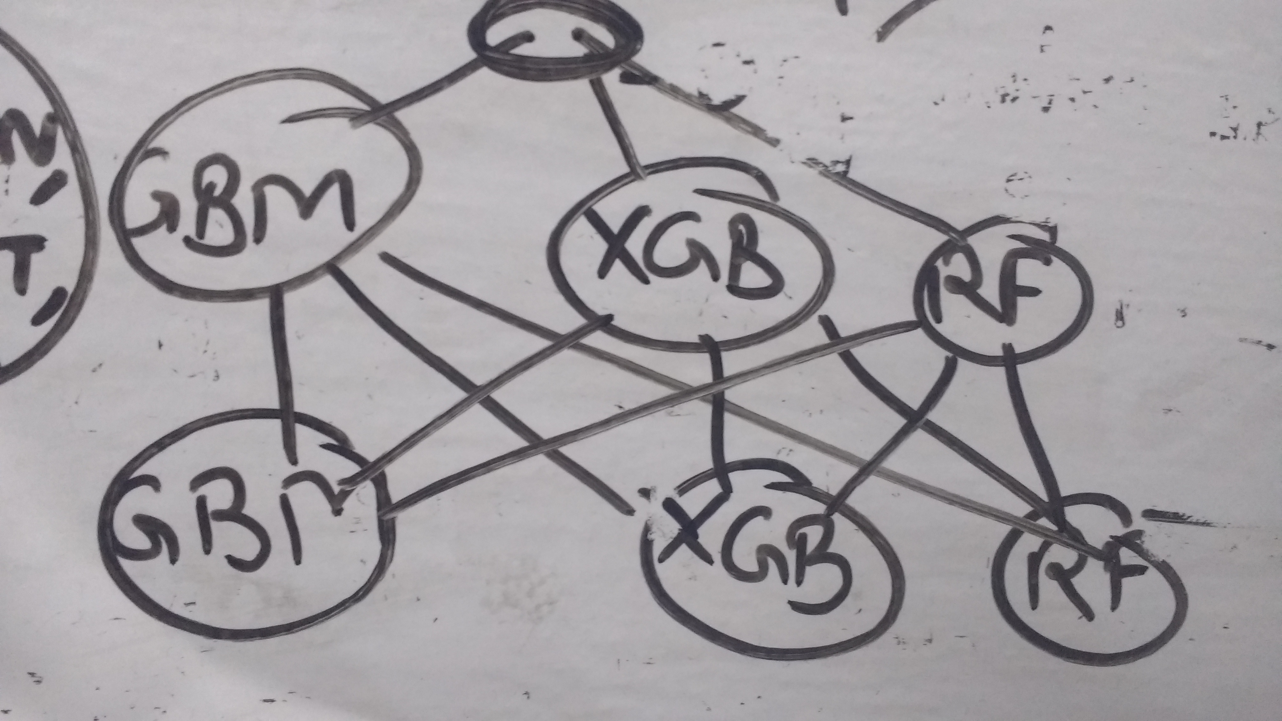
So, i had a 3-level stacker, but without a lot of diversity. The first two layers consisted of my 3 working models – XGBoost, GBM and RF. The third layer was a simple ensemble of the 2nd layer models. Probably, focussing more on the simpler models would’ve given me more diversity – i still got a decent 0.01 jump though :)

Note: For my final submission, I’ve averaged my submission with a brilliant public script. Everyone was doing it, probably ;)

Magic Features

In the last week of the competition, KazAnova, a very generous GrandMaster on Kaggle released an insanely powerful leak – The timestamps of image folders. Just plugging in the timestamp gave most people a 0.01 jump. I tried digging into the timestamp, its relation with the “created” variable etc – it is mostprobably an internal reason.

A similar magic feature was the listing_id contained in the image urls – Most of them were same as the original listing_id. Those which had different listings were probably reposts of the same apartment, which indicated it hadn’t got sold → “Low Interest”

Conclusions

My primary takeaways from the competition:

• Explore every variable. Each one of them. Look at the mean, median, max, outliers for numericals, and distribution for categoricals
• Spend most time on features. When you think you’ve got everything, start from scratch again.
• Build a systematic pipeline. It’s very easy to introduce leaks
• Build and test fast. Have efficient, fast, easy to tune algorithms for testing.
• Construct a model testing platform, stacking becomes easy.
• Spend a lot of time on Kaggle Kernels and Discussions. They’re damn cool :)

Overall, it was a fun couple of months! Learnt a lot, and this is just the launchpad for future competitions. Gonna get to that Top 10% soon :)

---